
This procedure is for inserting a new probe into the TT-AFM AFM and aligning the laser on it.
INSERT
- Remove the probe holder cassette from the instrument and place it, upside-down on probe insertion base, see figure 1.
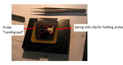
Figure 1: Probe holder cassette in Probe insertion base.
- Open box with probes, next to probe insertion base.
- Use probe tweezers to move probe to “landing pad” on probe insertion base.
- With one hand, push down on cassette until brass spring rises a little (it moves less than one millimetre). With your other hand, use rubber brush to move probe under spring, and then release. Check probe is seated all the way back in the slot.
- Lift probe cassette from probe insertion base, turn the right way up and slide into AFM instrument.
ALIGN
- If using a reflective sample, insert it now as it makes alignment easier.
- Start video microscope software, App300 .exe
- Push play button in app300.exe
- Locate probe in video microscope. This may be as simple as moving the focal plane of the microscope up and down using the wheel on the side.
10. If laser is not on, turn it on in AFM Workshop software. Also check, that motor is responding.[1]
11. Align laser on probe using the two laser translation thumbscrews located at the top and front of the AFM head; see figure 2.
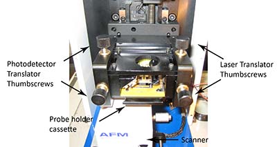
Figure 2: AFM Head, indicating location of thumbscrews for translation of laser and photodetector
12. For details on alignment of laser see page 89 of Eaton and West. Get the maximum signal. The laser may not look like a discreet spot, see figure 3.
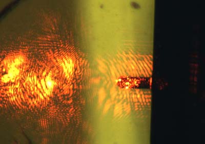
FIGURE 3: Laser alignment, often you get diffraction pattern instead of a visible spot
13. You may not be able to get the top-bottom(T-B) and left-right(L-R) signals to zero, without reducing the Top+Bottom, the important thing, is that they should change when you move the photodetector translation thumbscrews. Get the T-B and L-R signals as close to zero as you can (ideally within 0.1V), without jeopardising the T+B signal to do so.
This is all that is required, see the scanning protocol for beginning to scan.
[1] If either laser or motor does not respond, you need to turn of the software and ebox, then turn the ebox, then the software back on.
- Details
- Hits: 25490
- Scan (Vibrating Mode)
- Automated tip approach should have finished with the yellow line in the middle of the range , in the Z drive display. If not, approach again. If this never works, ensure the sample is not moving, and try reselecting the operation frequency.
- Go to “topo scan” tab.
- The table below has some suggested initial operating parameters. Some of these may be inappropriate for your sample. For example, you may only be interested in larger or smaller scans than 15 µm.
|
Parameter |
Suggested initial value |
|
type |
3d |
|
Scan rate |
0.5Hz |
|
Scan lines |
128 |
|
Scan size |
15µm |
|
Samples/pixel |
20 |
|
Rotation |
0 degrees |
|
center |
X and Y = 25 µm ( for 50 µm range) |
|
Gain |
2 |
|
Proportional |
200 |
|
Integral |
2000 |
|
Derivative |
0 |
|
Left image, Right Image |
Z_drive, Z_ampl |
- Click “start” to begin scanning.
- If your images show NOTHING (except laser interference in the amplitude channel), there are several things to try: reduce setpoint, approach again, and / or increase amplitude in prescan (in this order). Typically, the initial setpoint will be too high, so a reduction of 10 to 20% maybe required. Be cautious, and do not reduce setpoint below 60% of it’s initial value.
- Adjust parameters (especially scan speed, gain, Proportional, integral and Setpoint as required while scanning, watching the effect on the line scan and image. For more on this see chapter 4 of Eaton and West.
- Details
- Hits: 24795
The Requimte AFM Training Workshop will run during Easter 2014, from the 14th to 17th April. Following the successful courses that ran in 2011 and 2013, we've decided the course should run annually. The course includes several hours hands-on training in acquiring images with the atomic force microscope as well as AFM data processing. The course has been reorganised based on student feedback, and will feature advanced topics lectures from guest scientists in biology and materials science. This year, we plan to lengthen the practical part of the course, and hope to offer access to different instruments.
UPDATES:
- We are pleased to announce that this year, there will be 3 invited speakers, covering applications in a wide range of areas, and illustrating different capabilities of AFM:
Dr. Rui Rocha, CEMUP, Porto: "Materials Applications of AFM"
Dr. Simon Connell, University of Leeds, UK: "Dynamics in Biological AFM"
Dr. Filomena Carvalho, IMM, University of Lisbon, "Force Spectroscopy: Biological and Biomedical Applications"
Thanks to all the speakers for agreeing to talk.
- The provisional timetable can be downloaded here.
- There is a document containing in formation on travel to Porto, and hotels near the faculty of sciences here.
- The 2014 course has had all 16 places filled.
- The course flyer can be seen by clicking below:

A blog with information and student feedback from the 2013 course can be seen here: Requimte AFM Workshop 2013
Some information about the course that took place in 2011 can be seen here: http://atomicforceblog.blogspot.com/2011/09/2011-requimte-afm-mini-course.html
The course is sponsored by AFMWorkshop. It is also supported by The University of Porto, and will be integrated into the forthcoming network BIO-AFM.
- Details
- Hits: 27883
Approach (Vibrating Mode)
- Select “Vibrating”
- Ensure the Range Check is Complete (with green light) before approaching. DO range check with the probe somewhat close to the sample, so that you can see both sample and probe when range check is going on. During range check, the sample should translate around a square under the probe. If this does not happen, there is a problem.
- Moving the probe towards the sample is achieved with the Manual Z motor control buttons, “Up” and “Down”. It is recommended to use a speed less than half the maximum in this control. The best way to tell if the probe is approaching your sample, is to focus on the sample, and move the probe down until it is NEARLY in focus.
- Laser should already be aligned on probe, the place of the red dot on the photodetector is not very important. Ideally, TB should be in the middle of its range.
- The “vibrating” option makes the “Tune Frequency” window active.
- Use this window to find the resonant frequency of the probe, and set the correct amplitude:
- You should know the range of possible values of the natural resonant frequency (Rf) of your probe, if not, look on the box. For AppNano ACT probes, it-s 200-400kHz.
- Set “Lower” and “Upper” values accordingly to sweep this range. Note It won’t work if you have a “selected” value outside of the range.
- An initial guess for the driving amplitude (“Amplitude Vpp”), would be 0.4. You need at least 1 step per KHz, so for the above case, set steps to 200.
- Press “Sweep”
- You should see a sharp positive peak in the amplitude trace somewhere in that range (fig 4a). Move the green (lower), blue (selected) and red (upper) lines to close in on the peak. DO this by putting the green line on the left og the peak, the blue on in the middle of it and the red one on the right of the peak. Reduce the number of steps. Typically 50 steps would be a good choice.
- Repeat a sweep, with fewer steps (e.g. 50). Do this until the peak fills most to the windows as in figure 4b.
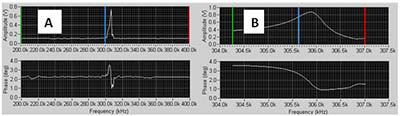
FIGURE 4 Tune window: A: Initial tune; B: Tune at scale suitable for selecting operating conditions.
- When you can see the peak clearly as in figure 4b adjust the Driving Amplitude (Vpp) to achieve the desired peak amplitude in the window, for example 1.0V.
- Now, the operating frequency should be chosen. Ideally, you will do this with the probe already close to the sample surface. If necessary, use “Down” button to achieve this, using the focus of the video microscope to help you get close.
- This guide assumes you use software version 1.5.6. Other versions will be different in this part of the procedure.
- Put the blue line on the highest point of the amplitude curve.
- Click system tab. Look at the amplitude value, it should be oscillating a little in the decimal points. Note the value.
- Go back to pre-scan window and move the blue line a little to the left. Check the amplitude value in system again. IF the amplitude increase, move a bit to the left again, and re-check. You want the amplitude to decrease by 2-5 % on moving left, compared to the maximum value. For example, if you have a maximum of 1.00V, look for a value of 0.95-0.98 V.
- NOTE: This procedure is particularly confusing because of a bug in the software, which means the REAL amplitude curve is shifted to the left of the DISPLAYED amplitude curve by ca.100Hz.
- Once you’ve done this, click “Lock Off”, which will turn to “Lock On”.
- Amplitude value will no longer oscillate.
- Ideally, you should start with a maximum amplitude between 1 and 1.2 V.
- Before automated tip approach you should get the probe as close to the sample as possible, without risking damage to the probe.
- Press “start” in the “automated tip approach” box.
- The approach occurs step by step , in the “woodpecker” method (see [i])
- Eventually, it should say feedback ON (green light).Ideally z drive should be in the centre of the range (0 V).
- If not in centre, press start again, and see if it goes to centre, if necessary try again.
- If something goes wrong with approach, it's possible the procedure will press the tip HARD against the sample, so it's always a good idea to watch the video microscope while approach is occurring. If you see cantilever bending, STOP, and raise the tip.
- Details
- Hits: 28606
This page contains currently a very small selection of the AFM images I have collected over the years. Please check back later to see more.
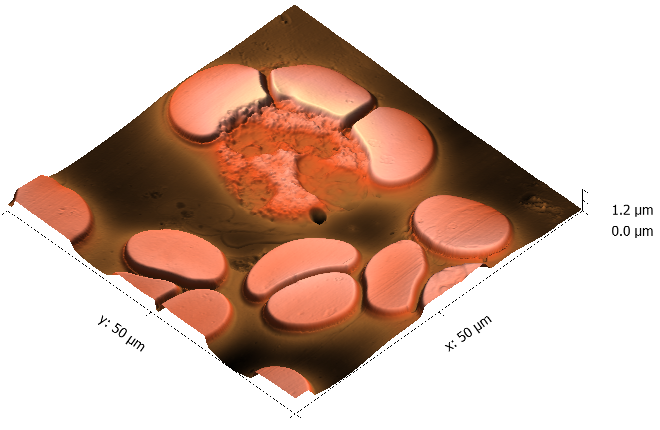
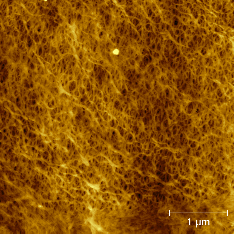
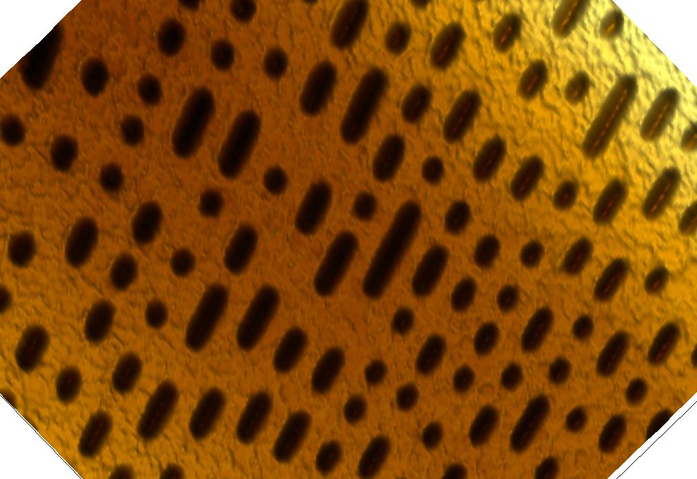
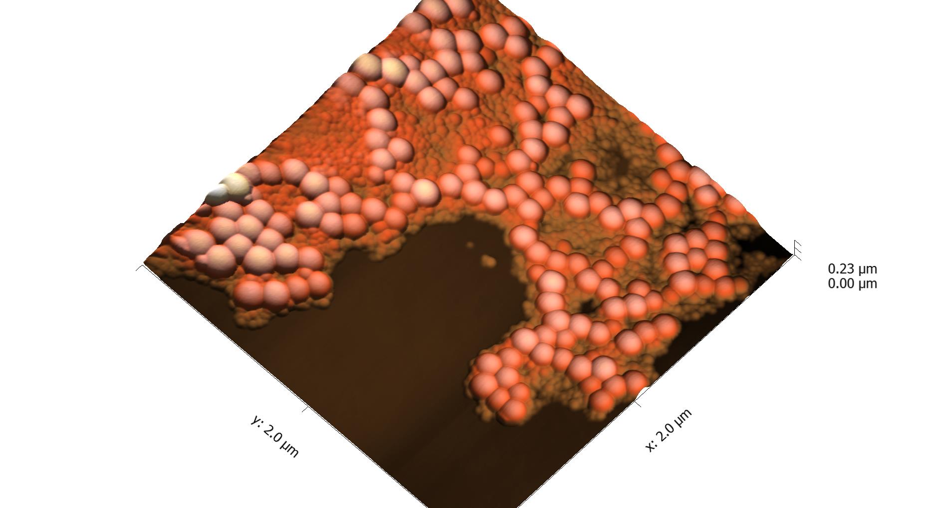
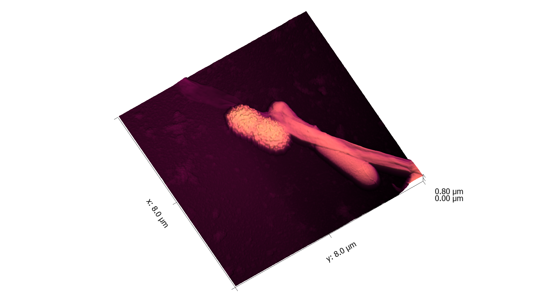
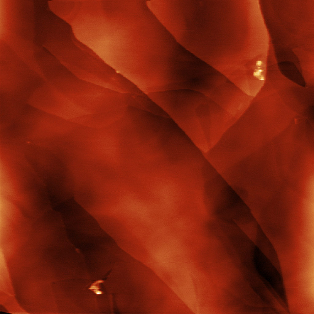
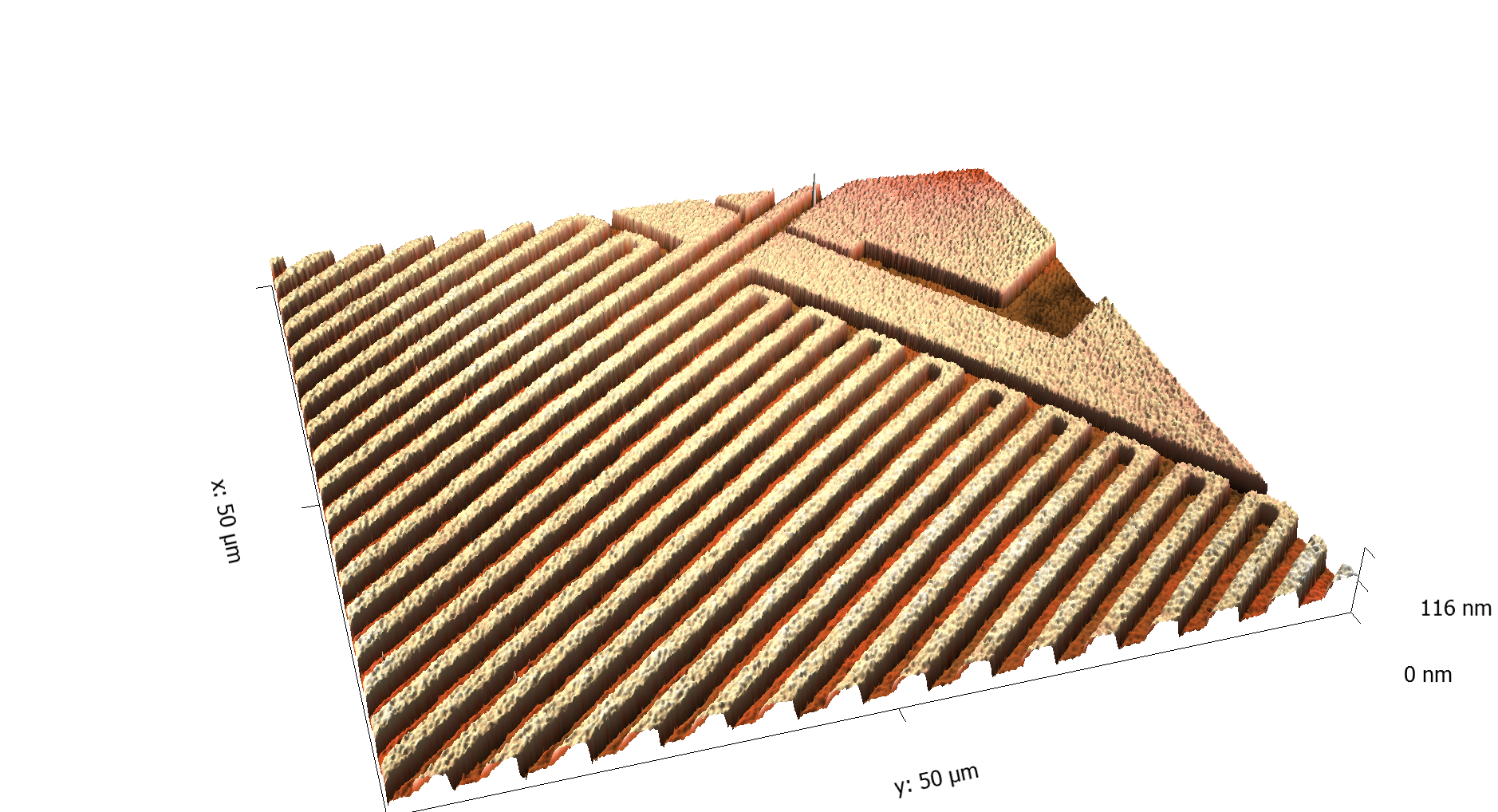
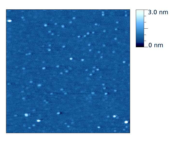
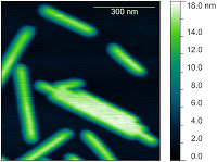
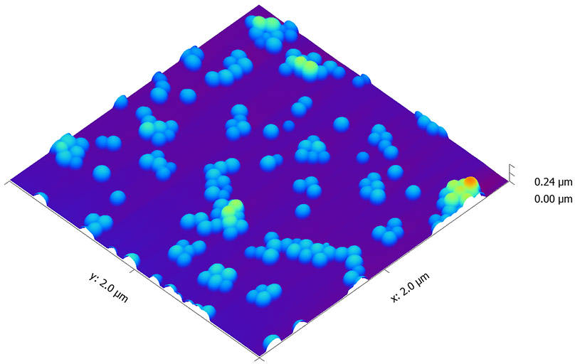


All images copyright 2010-2016, Peter Eaton, and may not be re-used without my permission
- Details
- Hits: 39254
Subcategories
Page 15 of 21